
The short answer
Why did the electron-scattering response point toward compact constituents inside a proton?
Read the evidence
Compare responses at different momentum transfers
The comparison is about how a measured quantity depends on the probe.
| Event class | Final-state condition | Historical inference |
|---|---|---|
| Elastic | Proton stays in its original state | Sensitive to an extended charge distribution |
| Highly inelastic | Hadronic final state can differ | Weak dependence helped support compact constituents |
| Scaling analysis | Compare defined structure functions | The chosen kinematic variables matter |
What elastic scattering preserves
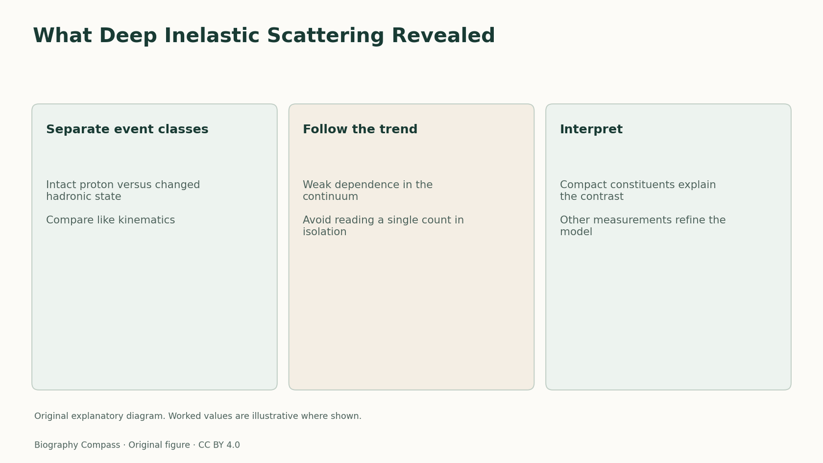
In elastic electron–proton scattering, the proton survives in its original internal state. Energy and momentum can be transferred to its overall motion, but the reaction has a constrained final state. At higher momentum transfer, the way charge is distributed inside the proton influences the probability of seeing such an event. A spatially extended distribution can produce a rapidly falling elastic response as the probe begins to distinguish smaller details. This provides a comparison for asking whether a different class of events behaves as if the electron had encountered much smaller objects.
What the inelastic continuum changes
In inelastic scattering the final hadronic system can have greater invariant mass than a proton. Rather than being restricted to a single elastic peak, the outgoing electron can be observed across a range of energies at a specified angle. The 1969 analysis distinguished the resonance region from a higher-excitation continuum and found weak dependence on momentum transfer there. That difference was suggestive because structureless point charges would not supply the same extended-target suppression as a proton that is required to remain intact. The distinction concerns a comparison of trends under specified conditions.
An invented normalized comparison
Imagine an elastic response dropping from 1.00 to 0.15 and then 0.03 as the momentum transfer increases in three steps. Suppose a suitably normalized inelastic response in a separate comparison is 1.00, 0.94 and 0.91. The second trend changes far less over those steps. These figures are invented and cannot be used to fit a proton model. They show why the informative observation is a dependence on the probe setting, rather than simply one large or small count. It still matters what was held fixed and how the electron-scattering factor was removed.
Sources for this section: [2]
Scaling uses a relationship between variables
The analysis compared structure functions built from measured cross sections. A scaling statement is more specific than saying that every rate is constant. It says that a combination of variables can capture much of the response over a tested range, leaving comparatively little additional dependence on another variable. Momentum transfer and energy transfer both enter the reasoning. A plot that changes both without saying how they are related is difficult to interpret. The 1969 study’s model assumptions and kinematic range should therefore be kept beside any concise statement of scaling.
What the evidence does and does not show
The observed pattern made a constituent picture experimentally compelling. It did not fix every property of those constituents or eliminate the need for other reactions and a more developed strong-interaction theory. Subsequent measurements could ask which structure functions scale, how the pattern changes at greater precision and how different targets compare. The historical accomplishment is precise without those extra claims. A collaboration measured electron response over several settings and showed that an intact, diffuse target was insufficient as the sole picture of what the electron encountered in highly inelastic events.
Continue the chronology
Related history guides
How the SLAC Spectrometer Measured Electrons
Read the spectrometer’s separate measurements of angle and momentum, and work through why collecting more tracks does not determine their directions.
Read the timeline1950sHow Electron Scattering Mapped Charge
Read how a proton’s elastic scattering response changes with momentum transfer, and work through an original example of phase cancellation.
Read the timelineBiography context
Explore United States through connected lives
Connected biographies
Researchers and collaborators
1930–
Jerome Friedman
Experimental particle physicistFollow Jerome Friedman from Chicago to Stanford and MIT, including Henry Kendall and Richard Taylor’s collaboration on deep inelastic electron scattering.Read biography1929–2018
Richard Taylor
Experimental physicist and accelerator researcherTrace Richard Taylor from Medicine Hat and Alberta to Stanford and Orsay, including the instruments that supported his SLAC–MIT scattering collaboration.Read biography1915–1990
Robert Hofstadter
Experimental physicist of electron scatteringFollow Robert Hofstadter from City College and Princeton to Stanford, where his collaborations used electron scattering to measure nuclear and proton structure.Read biographyQuick answers
Common questions
- What does inelastic mean here?
- Some energy and momentum can go into changing the internal hadronic state.
- Why compare more than one setting?
- A trend with momentum transfer can distinguish models that fit a single measurement.
Primary and institutional sources
How this history was checked
Dates, legal milestones and historical claims are checked against the official and institutional records below. This article was reviewed on 13 November 2026.