
The short answer
How did an instrument accept many electrons while still assigning an angle and momentum to each?
Read the evidence
Acceptance and resolution
An instrument can record a wide range while still determining where an event belongs.
| Property | Meaning | Why it matters |
|---|---|---|
| Acceptance | Which trajectories enter the detector | Controls available observations |
| Resolution | How well trajectories can be distinguished | Controls the precision of a reconstructed distribution |
| Calibration | How detector signals map to physical quantities | Allows comparison among instrument settings |
Two measurements for an outgoing electron
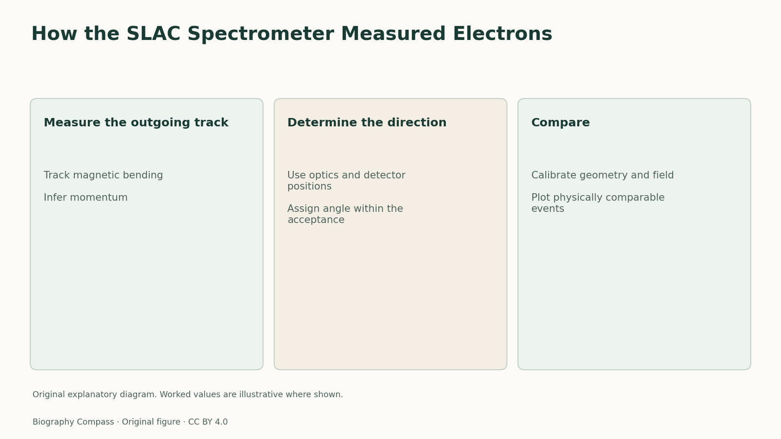
An electron arriving at a detector after a collision has a direction and a momentum. Both help establish how much energy and momentum it transferred. A magnetic spectrometer bends the trajectory of a charged particle. Given the field and a track measured through the instrument, that bending gives information about momentum. The direction at the target has to be reconstructed as well. In an experiment where rates change strongly with angle, uncertainty in that direction can matter as much as uncertainty in momentum. The instrument must keep the two measurements conceptually separate even if they use common hardware.
A large acceptance is not poor resolution by definition
Acceptance describes the range of trajectories that can enter and be recorded. Resolution describes how closely different true trajectories can be distinguished after they enter. Taylor’s facility account emphasizes this distinction. A practical spectrometer could accept a much wider angular range than the accuracy desired for assigning a particular event’s angle. Its optics and detectors therefore had to preserve enough information to infer the angle within that range. Simply narrowing the opening would lose useful tracks. Simply accepting them without reconstructing their directions would wash out the angle dependence being studied.
Sources for this section: [1]
An invented track comparison
Suppose a detector accepts incoming tracks over ten arbitrary units of angle and can place each reconstructed track into bins one unit wide. A second detector accepts the same ten-unit range but records only the total number. They collect similar ranges yet support different analyses. The first can distinguish events near one edge from events near the centre. The second cannot reconstruct that distribution after the fact. These values are illustrative, not SLAC specifications. The comparison shows why a paper needs to describe what is reconstructed, in addition to how many events the apparatus registers.
Sources for this section: [1]
Check geometry and momentum calibration
The relation between measured position and outgoing angle depends on the instrument geometry. The relation between magnetic bending and momentum depends on the field and the known trajectory through it. Taylor’s lecture describes the design requirements and early commissioning with elastic scattering. A process with a well-constrained relationship between angle and outgoing energy can help expose a miscalibration. At the same time, calibration in one region does not guarantee equal performance everywhere. Large instruments require checks over relevant settings, especially when an analysis compares results taken at different angles or momenta.
From a detector track to a scattering plot
The historical paper reports scattering cross sections after the collaboration turned tracks into physical variables and accounted for the measuring apparatus. A result expressed as a function of momentum transfer cannot be read directly from an uncalibrated detector image. Keeping the measuring chain visible makes the final comparison easier to audit. Start from the angle and momentum of each detected electron, apply the defined geometry and calibrations, and then compare how the inferred distributions change under stated conditions. That is the separate achievement of the spectrometer programme underlying the more famous interpretation about proton constituents.
Continue the chronology
Related history guides
What Deep Inelastic Scattering Revealed
Read the 1969 SLAC–MIT analysis, distinguish elastic and inelastic scattering, and compare illustrative responses at several momentum transfers.
Read the timeline1950sHow Electron Scattering Mapped Charge
Read how a proton’s elastic scattering response changes with momentum transfer, and work through an original example of phase cancellation.
Read the timelineBiography context
Explore Stanford, California, United States through connected lives
Connected biographies
Researchers and collaborators
1929–2018
Richard Taylor
Experimental physicist and accelerator researcherTrace Richard Taylor from Medicine Hat and Alberta to Stanford and Orsay, including the instruments that supported his SLAC–MIT scattering collaboration.Read biography1930–
Jerome Friedman
Experimental particle physicistFollow Jerome Friedman from Chicago to Stanford and MIT, including Henry Kendall and Richard Taylor’s collaboration on deep inelastic electron scattering.Read biography1915–1990
Robert Hofstadter
Experimental physicist of electron scatteringFollow Robert Hofstadter from City College and Princeton to Stanford, where his collaborations used electron scattering to measure nuclear and proton structure.Read biographyQuick answers
Common questions
- Can an acceptance range replace the angle measurement?
- It establishes which tracks could be seen, not their individual directions.
- Why use an elastic reaction during commissioning?
- Its constrained kinematics can provide a check on how the instrument reconstructs angle and energy.
Primary and institutional sources
How this history was checked
Dates, legal milestones and historical claims are checked against the official and institutional records below. This article was reviewed on 13 November 2026.