
The short answer
How did an unexpected mark on a survey chart become evidence for a new astronomical source? Compare selected original journal pages with two participants’ later accounts, then distinguish pulse timing, frequency delay and a physical explanation.
Original source comparison
Ask which inference a test can support
A series of corroborating observations is more informative than treating regularity as a complete explanation.
| Country | What the evidence supports | What it does not establish |
|---|---|---|
| Recurring celestial position | A source tracks the sky rather than an arbitrary local schedule. | Every terrestrial explanation eliminated without other tests. |
| Reception by other equipment | Evidence against a defect limited to one receiver system. | A unique physical model for the emitter. |
| Frequency-dependent delay | A basis for investigating dispersive propagation. | That the lag equals the interval between successive pulses. |
| 1968 stellar discussion | The authors considered compact-star explanations with stated uncertainty. | That the later rotating-neutron-star model was already settled. |
| 1974 Nobel citation | Identifies the award recipients and specified recognition. | A complete list of everyone who contributed to the 1968 paper. |
Chronology
A timeline of the turning points
Survey begins
The array begins observations for the compact-source survey.
Resolved pulses
Fast recording reveals regularly spaced pulses.
Printed receipt date
The original journal article records this receipt milestone.
Publication
The five-author Nature paper reports the source and further candidates.
Retrospective lecture and award
Hewish’s lecture discusses subsequent interpretation; Ryle and Hewish receive the Nobel Prize.
The telescope had a different original purpose
The Cambridge array was built to study compact radio sources through interplanetary scintillation. The original Nature report describes observations at 81.5 MHz, with 2,048 dipoles arranged in sixteen rows of 128 and four receiving beams. Hewish planned the instrument; Bell helped construct it and analysed its charts. This purpose matters because an unexpected signal could easily be classified as a defect or interference in a survey designed for another phenomenon. The discovery required understanding ordinary records well enough to identify something that did not fit them. Repeated sky coverage supplied opportunities to test whether the feature returned at a consistent celestial position.
An initial feature was not yet a measured pulse train
Bell’s later interview dates a surviving early signal record to 6 August 1967 and the first resolved pulses to 28 November. The paper describes 13 August as the earliest record suitable for a particular position measurement. These need not be competing dates for the same event: detection, a usable positional record and resolved periodicity are different achievements. The slower survey record could reveal an unusual feature while obscuring its detailed timing. Faster recording and follow-up observations changed what could be inferred. Avoid compressing the whole process into a single dramatic moment when a fully explained new star supposedly announced itself.
Different checks addressed different alternatives
The source’s recurrence at a celestial position helped test a terrestrial-interference explanation. Reception using other equipment reduced the chance of a fault confined to one instrument. Accurate timing revealed systematic effects associated with the Earth’s motion. Frequency-dependent arrival delays provided another line of evidence concerning propagation through intervening plasma. In her retrospective account, Bell assigns work on dispersion and receiver tests to Pilkington, Scott and Collins. The first paper names all five authors. These checks are complementary: observing a regular pulse alone would not, without context, prove either an extraterrestrial source or a particular kind of star.
Pulse period, arrival delay and pulse width are not interchangeable
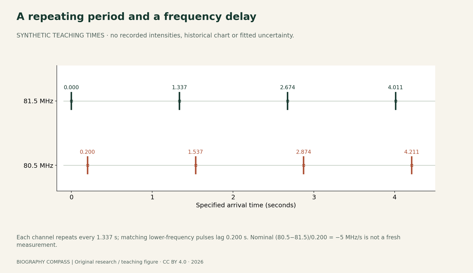
The original paper reports a repetition interval of about 1.337 seconds. Its figure and discussion compare receivers at 81.5 and 80.5 MHz, with the lower-frequency pulse arriving about 0.2 seconds later. Those are different measurements: the first compares successive pulses at one frequency; the second compares one event across two frequencies. The authors also distinguish the broadened recorded feature from the much shorter pulse duration inferred under narrower frequency conditions. A reader who calls every timescale the star’s period would confuse recurrence, propagation and instrumental response. The report explicitly discusses tests of the frequency behaviour rather than treating one trace as a complete explanation.
Sources for this section: [1]
Try a declared synthetic timing example
The teaching figure is newly generated and contains no copied chart or measured intensity data. Set four high-frequency arrival times to 0, 1.337, 2.674 and 4.011 seconds. Set the matching lower-frequency times to those values plus 0.200 seconds. What are the three successive intervals in each channel? What is the lag between matching pulses? If the frequency changes from 81.5 to 80.5 MHz over that lag, what signed change per second does this simplified pair imply? Finally, decide whether a constant lag proves that the source is an artificial transmitter, a white dwarf or a rotating neutron star.
Sources for this section: [1]
Reference answer: the same period can accompany a frequency lag
Both channels have intervals of 1.337 seconds, and each lower-frequency arrival is delayed by 0.200 seconds. The simplified frequency change is (80.5−81.5)/0.200=−5 MHz per second. This reproduces the scale of the paper’s frequency-sweep discussion using specified teaching values; it is not a fresh fit to its original records or an uncertainty estimate. A positive arrival lag does not make the recurrence period 0.200 seconds. Nor does the arithmetic by itself choose the emitting object. A propagation interpretation needs the observational tests, and a stellar model needs further physical arguments and evidence.
Sources for this section: [1]
The first report left the physical interpretation open
The article, published on 24 February 1968, discusses white-dwarf or neutron-star oscillations as possible explanations. It does not present the later rotating-neutron-star lighthouse interpretation as already demonstrated. Hewish’s 1974 lecture describes the subsequent development, including Thomas Gold’s rotation proposal and evidence from the Crab pulsar. That retrospective view contains information unavailable to the first paper’s authors at publication. Keeping the stages separate makes the discovery more intelligible: observations can be robust enough to establish a new phenomenon while the best explanation is still changing. A later successful model should not be written backwards into every sentence of the original report.
Authorship, recollection and prizes answer different questions
The paper lists A. Hewish, S. J. Bell, J. D. H. Pilkington, P. F. Scott and R. A. Collins and acknowledges additional discussion and funding. Its printed receipt date is 9 February 1968. Participant recollections provide richer accounts of work and decisions but were written later and sometimes compress dates. The 1974 Nobel award went to Ryle and Hewish, with different citations; it is a record of the committee’s selection, not a substitute author list for the discovery paper. Read Bell’s persistence, Hewish’s survey and follow-up role, and colleagues’ tests as specific contributions. This guide compares selected acquired pages and accounts; it does not claim access to the complete laboratory notebooks.
Connected biographies
People behind the work

1943–present
Jocelyn Bell Burnell
Astrophysicist, teacher and research leaderJocelyn Bell Burnell recognised unusual radio signals while analysing a Cambridge sky survey and pursued the evidence that led to pulsars. Her later work crossed astronomical wavelengths, teaching and institutional leadership; she used a major science prize to support researchers from underrepresented groups.Read biography1924–2021
Antony Hewish
Radio astronomer and instrument designerAntony Hewish developed ways to use radio scintillation to study intervening plasma and compact sources. His survey instrument became the setting for Jocelyn Bell’s recognition of pulsars, followed by team observations and a Nobel Prize shared with Martin Ryle.Read biographyQuick answers
Common questions
- Were the signals originally proved to be alien messages?
- No. Artificial explanations were considered and tested; the report investigated a natural astronomical source.
- Is the figure an original pulsar recording?
- No. It is a labelled synthetic timing exercise using specified values, not copied historical chart data.
Primary and institutional sources
How this history was checked
Compare the identified original texts, participant accounts and institutional records; the teaching examples are separately labelled. This article was reviewed on 27 October 2026.
- Hewish and colleagues; Pennsylvania State University course-hosted copyOriginal 1968 Nature article scan, with later contributor cover sheet
- A. Hewish, S. J. Bell, J. D. H. Pilkington, P. F. Scott and R. A. CollinsObservation of a Rapidly Pulsating Radio Source, Nature 217, 709–713 (1968)
- Antony Hewish; Nobel FoundationPulsars and High Density Physics, Nobel Lecture, 12 December 1974
- S. Jocelyn Bell Burnell; Cosmic Search, reproduced by NRAOLittle Green Men, White Dwarfs or Pulsars? Retrospective account
- University of Cambridge; interview by Louise WalshJourneys of discovery: Jocelyn Bell Burnell and pulsars
- Nobel FoundationThe Nobel Prize in Physics 1974: recipients and citation