
The short answer
A quadratic can expose a parameter boundary without proving the spacetime in which it appears. Keep the equation, its coordinate meaning and a claim about a collapsing body separate.
Evidence and original analysis
One equation, three root cases
The dimensionless parameter values are invented.
| Stipulated α | Real roots x | Coordinate separation Δx |
|---|---|---|
| 0.6 | 0.2 and 1.8 | 1.6 |
| 1 | 1 (repeated) | 0 |
| 1.2 | None | Not defined for real roots |
Chronology
A timeline of the turning points
Selected record
Historical scope for this question.
Original exercise
Invented inputs and analysis, not reconstructed observations.
A calculation inside a larger geometry
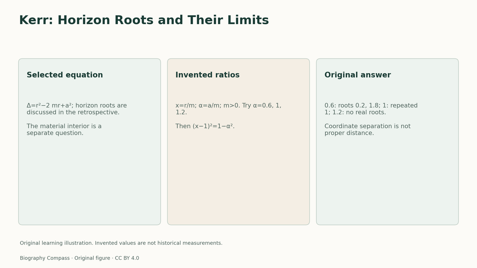
Kerr’s retrospective gives Δ=r²−2 mr+a² and identifies the two horizon surfaces with its roots. It also warns that a coordinate radius is not a description of where all the matter lies.
Here m is the mass parameter and a the rotation parameter.
This guide reads the later account, not the original discovery letter. Its explicit reservations matter: the existence of an exact geometry does not itself supply a material model of stellar collapse.
Sources for this section: [1]
An original dimensionless comparison
Set x=r/m and α=a/m, with m>0. Dividing the stated polynomial by m² gives x²−2x+α²=0. These ratios remove the need to assign an SI mass or length; no astronomical measurement is supplied. Restrict this exercise to α≥0.
Invent three cases, α=0.6, 1 and 1.2. Complete the square, find all real roots, and calculate their coordinate separation where they exist. What can the root calculation alone establish?
Sources for this section: [1]
Reference answer
Completing the square gives (x−1)²=1−α², so x=1±sqrt(1−α²). For α=0.6 the square root is 0.8 and the roots are 0.2 and 1.8. Their separation is 1.6 in x, or 1.6 times m in the original radial coordinate.
For α=1 the root is repeated at x=1, with zero separation. For α=1.2 the right side is −0.44, so there are no real roots of this polynomial. That result does not say that every mathematical spacetime or every physical phenomenon disappears.
The threshold follows from the sign of 1−α². None of these coordinate differences is a measured proper distance; calculating one would require the metric and a specified path or slice.
Sources for this section: [1]
Read the conditional result accurately
The exercise derives the algebraic boundary from the stated equation. It does not derive that equation from Einstein’s field equations, prove that its surfaces are event horizons, or simulate the formation of a rotating star. Those are additional geometric and physical questions. The original calculation is useful precisely because its answer does not pretend to settle them.
Sources for this section: [1]
Continue the chronology
Related history guides
Biography context
Explore New Zealand through connected lives
Connected biographies
Researcher and context
Quick answers
Common questions
- Are these observed black-hole parameters?
- No. They are original dimensionless inputs.
- Do no real roots invalidate the entire metric?
- No. This calculation tests only the stated polynomial’s real-root condition.
Primary and institutional sources
How this history was checked
Selected record passages ground the historical explanation. Original fixtures and answers are labelled separately. This article was reviewed on 31 October 2026.