
The short answer
How did a narrow feature in radio frequency identify hydrogen in the Milky Way?
Read the evidence
What can be learned from a line
Identification, velocity and brightness depend on different features of the measurement.
| Feature | Role | Additional requirement |
|---|---|---|
| Rest frequency | Identifies a physical transition | Compare with the observed feature |
| Observed shift | Can indicate line-of-sight motion | Calibrate the frequency scale |
| Line strength and shape | Characterize the detected emission | Account for baseline and sensitivity |
An atom can emit at a characteristic frequency
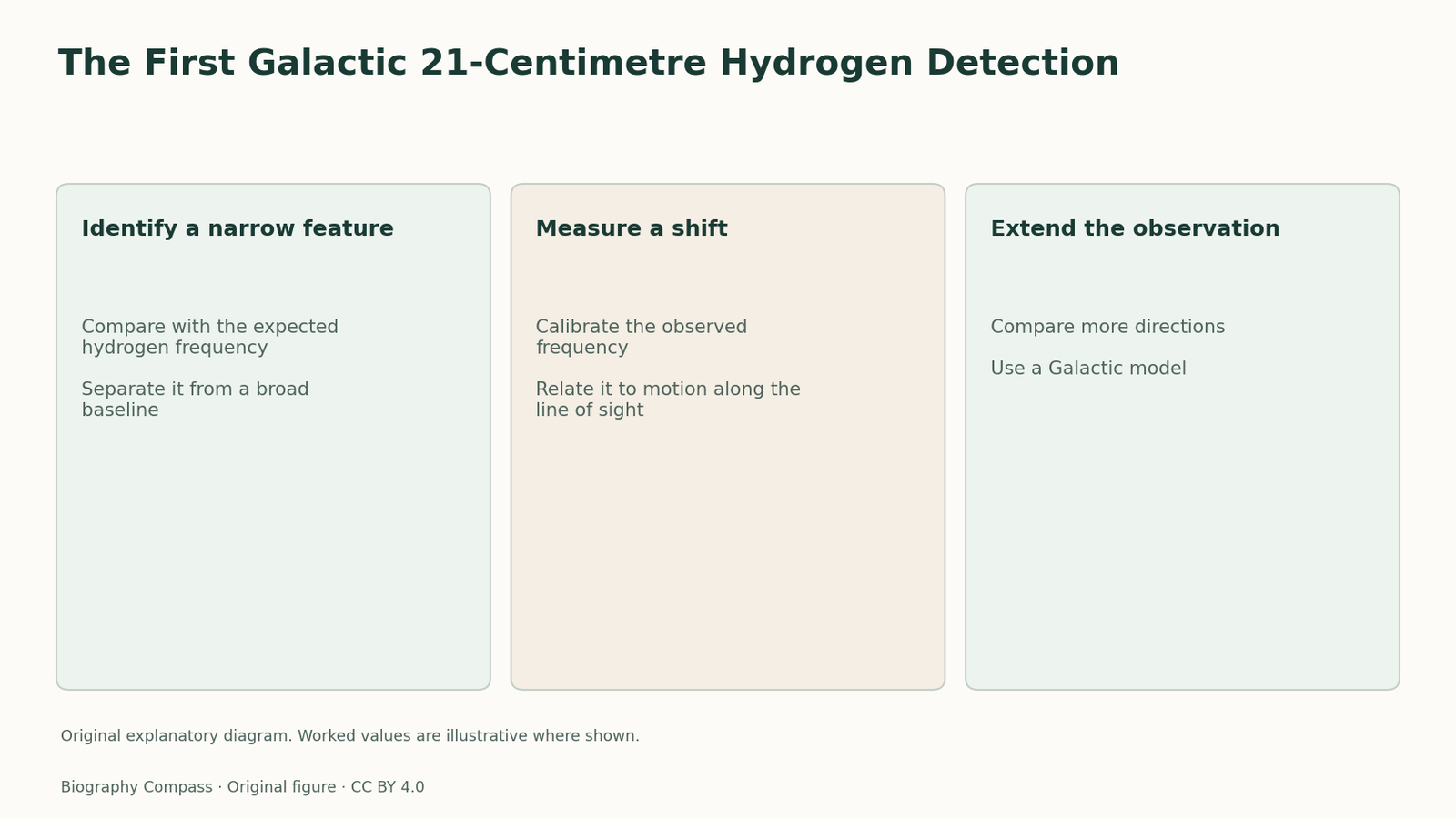
Neutral hydrogen has closely spaced magnetic states associated with the relative spins of its electron and proton. A transition between those states can emit radio radiation. The frequency is near 1,420 megahertz, corresponding to a wavelength of about 21 centimetres. An astronomical receiver looks for additional power near this characteristic frequency. Unlike a broad rise in receiver noise, a line is a feature localized in frequency. The line shape and centre can also be affected by motion and by the range of velocities among the emitting atoms. Identification begins by finding the expected kind of feature.
One line can sit on a broad baseline
Ewen and Purcell’s 1951 report concerns detection of Galactic hydrogen radiation. To interpret such a result, a reader needs to separate a frequency-dependent feature from a broad background or slowly changing instrumental response. A signal confined to a narrow range is stronger evidence of a transition if it has the expected frequency and survives checks on the receiver. The direction of observation also matters. Radio measurements of different parts of the sky can change the contribution from Galactic material. A feature in an electronics component may respond differently to those comparisons.
Sources for this section: [1]
An invented receiver reading
Imagine five adjacent frequency bins with power values 10, 10, 15, 11 and 10 in arbitrary units. A broad change adding three units to every bin would raise the baseline but leave the central excess visible. A second observation showing a feature at a slightly shifted frequency could contain information about motion, provided the frequency reference is known. These values are invented. A real identification needs estimates of noise and the instrument’s frequency response. The exercise separates the question of whether a line is present from the later question of what its shape or displacement implies.
Sources for this section: [1]
From detection to motion
The line’s position can change because emitting gas moves along the line of sight. Measuring such changes across different directions can help infer Galactic rotation, but that analysis requires a model for the geometry and the distribution of gas. The separate 1951 report by Muller and Oort addressed the rotation question. The relationship between the publications is valuable because a newly detected line supplied a tool for additional astronomy. It was not equivalent to having measured all Galactic motions in the initial detection. A velocity inference needs an identified rest frequency and other observational information.
How to read the achievement
Keep three quantities separate: the frequency at which an atomic transition occurs at rest, the frequency at which a receiver observes it and the strength of the line relative to its surroundings. The first helps identify the source. The second can convey motion. The third relates to the detected emission and instrument sensitivity. Those distinctions turn a brief historical report into a way of reading a spectrum. The 1951 collaboration matters because it gave astronomers a measurable radio feature from a widespread constituent of the Galaxy, making later maps and comparisons possible.
Continue the chronology
Related history guides
The Excess Antenna Temperature of 1965
Read the 1965 Bell Labs antenna measurement alongside the Princeton interpretation, with an original noise-budget example that isolates an excess.
Read the timeline1970–1992How COBE DMR Measured Differences in the Sky
Read the first-year COBE maps, compare two independent receiver channels, and see how smoothing and Galactic masks qualify the reported sky signal.
Read the timeline1946How Nuclear Induction Turned Spin into a Signal
Read the 1946 water experiment and use an original geometry comparison to see how precessing magnetization can induce a signal in a coil.
Read the timelineBiography context
Explore United States through connected lives
Connected biographies
Researchers and collaborators
1912–1997
Edward Purcell
Experimental physicist of magnetic resonance and radio astronomyFollow Edward Purcell from Purdue and Harvard to magnetic resonance and the 1951 detection of neutral hydrogen radiation with Harold Ewen.Read biography1905–1983
Felix Bloch
Theoretical and experimental physicistFollow Felix Bloch from Zurich and Leipzig to Stanford, including his collaboration with Hansen and Packard on detecting magnetic resonance by induction.Read biography1933–2024
Arno Penzias
Radio astronomer and Bell Labs research leaderRead Arno Penzias’s path from Germany to Columbia and Bell Labs, including the unexplained antenna signal and collaboration with Robert Wilson.Read biographyQuick answers
Common questions
- Why call it the 21-centimetre line?
- That is the approximate wavelength corresponding to the hydrogen transition’s radio frequency.
- Does finding the line itself map Galactic rotation?
- Rotation requires measurements across directions and a model that relates frequency shifts to motion.
Primary and institutional sources
How this history was checked
Dates, legal milestones and historical claims are checked against the official and institutional records below. This article was reviewed on 13 November 2026.