
The short answer
How can microscopic differences become less important when a system is viewed over greater distances?
Read the evidence
How a parameter changes under rescaling
The illustrative multipliers show distinct directions of change near a fixed point.
| Case | After repeated rescaling | Interpretation |
|---|---|---|
| Growing perturbation | 0.02 becomes 0.16 | Relevant in the illustration |
| Shrinking perturbation | 0.02 becomes 0.0025 | Its effect diminishes |
| Shared exponent | Models approach the same relevant fixed point | Microscopic amplitudes can still differ |
One description at several scales
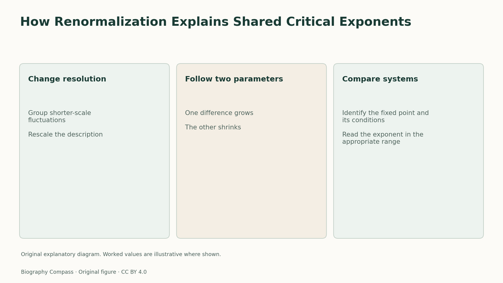
Near some continuous transitions, a region of material can show correlated fluctuations across many distances. Examining only isolated microscopic pieces does not reveal how those regions fit together. The renormalization group compares descriptions at successive resolutions. Grouping nearby degrees of freedom can change the numerical parameters used in the coarse description. Rescaling then lets a researcher compare the new description with the old one. A fixed point represents a description whose relevant form remains unchanged under that procedure, rather than a claim that the material has stopped fluctuating.
Relevant and irrelevant changes
Imagine two models that differ slightly from the same fixed point. One difference may grow when the description is repeatedly rescaled. Another may shrink. A growing difference is relevant to the large-scale behaviour and may need to be tuned to see critical behaviour. A shrinking difference can become difficult to detect in long-distance observations. The distinction explains why changing some microscopic details may leave a large-scale exponent nearly unchanged while changing symmetry or dimension can lead to another class. Identifying the direction of change is more informative than simply saying that the models resemble each other.
An illustrative iteration
Suppose an invented transformation doubles a small change in parameter A and halves a small change in parameter B. Starting both at 0.02, three steps leave A at 0.16 and B at 0.0025. Those values are not measured properties of a material. They show that two equally small initial differences can have very different effects after coarse-graining. A real calculation must justify which variables are being transformed and how the multipliers are obtained. The linearized comparison is also meant near the fixed point, where the approximation may cease to hold if a growing difference becomes large.
What a critical exponent measures
A critical exponent describes a power-law dependence near a transition, such as how a characteristic length changes when temperature approaches its critical value. The renormalization-group argument connects that behaviour to the way disturbances grow or shrink with scale. Different systems can share exponents if their large-scale descriptions approach the same fixed point in the relevant sense. They need not share the same transition temperature or the same numerical amplitude. An experiment comparing universality should specify which exponent is estimated and whether its measured region is close enough to the transition for asymptotic behaviour to be expected.
Use the analogy with a measured range
A reader should separate the microscopic model, the transformation and the exponent reported at the end. A coarse description can suppress some detail without erasing every physical difference. The comparison is meaningful if the transformation respects the features that matter and if the system is observed in the appropriate scale range. In a real sample, finite dimensions or a limited temperature window can change an apparent power law. This is why the fixed-point picture explains a pattern in data rather than promising identical behaviour everywhere for all systems that look superficially similar.
Continue the chronology
Related history guides
Why the TKNN Hall Conductance Is an Integer
Read the conditions of the 1982 Hall conductance result, then use a winding-number analogy to understand why a gap can protect an integer.
Read the timeline1981–1983Haldane’s Gap and the Spin-Chain Divide
Compare the low-energy spectrum of integer and half-integer antiferromagnetic chains, and use a finite-size example to test what counts as a gap.
Read the timeline1972–1973Vortex Pairs and a Two-Dimensional Transition
Follow the energy and entropy of vortices, compare paired and free defects, and work through a simplified free-energy estimate for a larger system.
Read the timelineBiography context
Explore United States through connected lives
Connected biographies
Researchers and collaborators
1936–2013
Kenneth Wilson
Theoretical physicist of critical phenomenaRead Kenneth Wilson’s path from Harvard and Caltech to Cornell and Ohio State, including how he developed scale-based methods for critical phenomena.Read biography1943–
Michael Kosterlitz
Theoretical physicist of phase transitionsFollow Michael Kosterlitz from Aberdeen through Cambridge, Oxford and Birmingham, including his work with David Thouless on two-dimensional phase transitions.Read biography1951–
Duncan Haldane
Theoretical physicist of quantum matterFollow Duncan Haldane’s path from Cambridge and Grenoble to Princeton, including Philip Anderson’s mentorship and his prediction for spin chains.Read biographyQuick answers
Common questions
- Can two materials share an exponent and have different transition temperatures?
- They can share the large-scale power-law form while differing in other quantities.
- Why track several scales?
- The way a difference grows or shrinks can reveal which physical features control the large-scale response.
Primary and institutional sources
How this history was checked
Dates, legal milestones and historical claims are checked against the official and institutional records below. This article was reviewed on 13 November 2026.