
The short answer
Two measurements can move together, and a change of units can make a raw distance look very different. A small fictional model lets you check both effects without using a historical human dataset.
Original worked comparison
Read the conditions alongside the result
All numerical examples in this table are invented teaching cases. They are not historical measurements.
| Case | Calculation or observation | Conclusion and limit |
|---|---|---|
| Original vector | d=(2,3); squared score 1.5. | Use the supplied S, not a diagonal replacement. |
| Converted vector | d=(200,3); converted-covariance score 1.5. | Raw squared length changes to 40,009. |
| Opposite signs | d=(2,−3); squared score 3. | Equal raw length does not imply equal quadratic score. |
Chronology
A timeline of the turning points
Supply a covariance
Use the explicitly invented matrix and vector.
Find the inverse
Check determinant 32 before multiplication.
Transform both inputs
Convert vector and covariance in compatible units.
State the technical definition before substituting numbers
Chaudhuri’s 2020 review gives D²=ΔᵀΣ⁻¹Δ, where Δ is the difference between means and Σ is their common nonsingular covariance matrix. This squared distance accounts for the covariance structure, instead of simply adding squared coordinate differences.
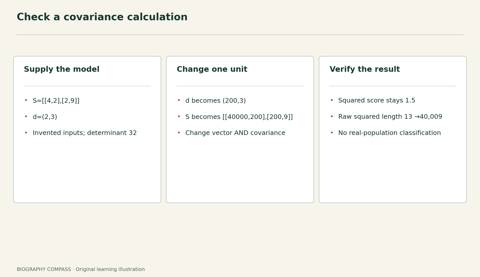
For the invented example, supply covariance matrix S=[[4,2],[2,9]] and a difference vector d=(2,3). S is symmetric, its first diagonal entry is positive and its determinant is 32, so this two-dimensional covariance model is positive definite. These supplied values have no connection with an observed population.
Sources for this section: [1]
Calculate before converting the units
The inverse is S⁻¹=(1/32)[[9,−2],[−2,4]]. Multiplying out gives dᵀS⁻¹d=(9×2²−4×2×3+4×3²)/32=48/32=1.5. This is the squared score. Its square root is approximately 1.225; reporting 1.5 as the unsquared distance would change the quantity.
For comparison, raw squared Euclidean distance is 2²+3²=13. If the off-diagonal entries were replaced by zero while keeping the supplied variances, the weighted squared score would be 2²/4+3²/9=2. That is a changed model, not an alternative calculation using the original covariance.
Sources for this section: [1]
Convert the vector and the covariance together
Rescale only the first measurement by 100. The new difference is (200,3), and the covariance becomes [[40000,200],[200,9]]. The first variance changes by 100², while each cross-covariance changes by 100. Applying the same quadratic calculation gives 1.5 again. Raw squared Euclidean distance instead becomes 40,009.
The invariance holds because both the measurements and their covariance were transformed consistently. Converting the vector while leaving the original covariance matrix unchanged would mix units. It would not be a valid test of this model. Replacing or estimating the covariance differently is another change that should be disclosed.
Sources for this section: [1]
Exercise: equal raw lengths, different directions
Keep the original S and compare d₊=(2,3) with d₋=(2,−3). Both have raw squared length 13. Calculate the quadratic score for the second direction, then explain what the comparison establishes.
Reference answer: the second numerator is 36+24+36=96, giving a squared score of 3. The first score was 1.5. The sign change affects the cross term even though the raw lengths match. Under this supplied covariance, direction matters. The calculation does not prove that a real observation is abnormal, assign a causal explanation or validate an estimated covariance matrix.
As a final check, distinguish the assumptions from the outputs: the matrix and vectors were supplied; the inverse and scores were derived. A real application would need suitable measurements and a justified covariance estimate. No human classification, historical result or probability threshold is inferred from this exercise.
Sources for this section: [1]
Continue the chronology
Related history guides
Biography context
Explore India and international statistical research through connected lives
Connected biographies
People connected with this question
1893–1972
Prasanta Chandra Mahalanobis
Statistician and institution builderMahalanobis connected statistical research with institutions, national surveys and planning.Read biography1920–2023
C. R. Rao
Statistician and teacherC. R. Rao combined theoretical statistics with research training, institutional leadership and later American appointments during a career spanning several generations.Read biographyQuick answers
Common questions
- Is 1.5 the distance or its square?
- It is the squared score in this example; the distance is its square root, approximately 1.225.
- Does the example prove that a real observation is an outlier?
- No. It supplies invented values and no validated probability threshold or real covariance estimate.
Primary and institutional sources
How this history was checked
Historical and technical records ground the context. The numbered examples and reference answers are original teaching material; their invented values are identified in the text. This article was reviewed on 29 October 2026.