
The short answer
A measurement tells us something at a particular time and under particular conditions. Predicting where an object will be requires an additional model and a way to estimate its parameters.
Compare the representations
Why is a tracking observation different from an estimated orbit or a future prediction?
Keep the stated evidence separate from the conclusions it permits.
| Distinction | Representation or action | What follows — and what does not |
|---|---|---|
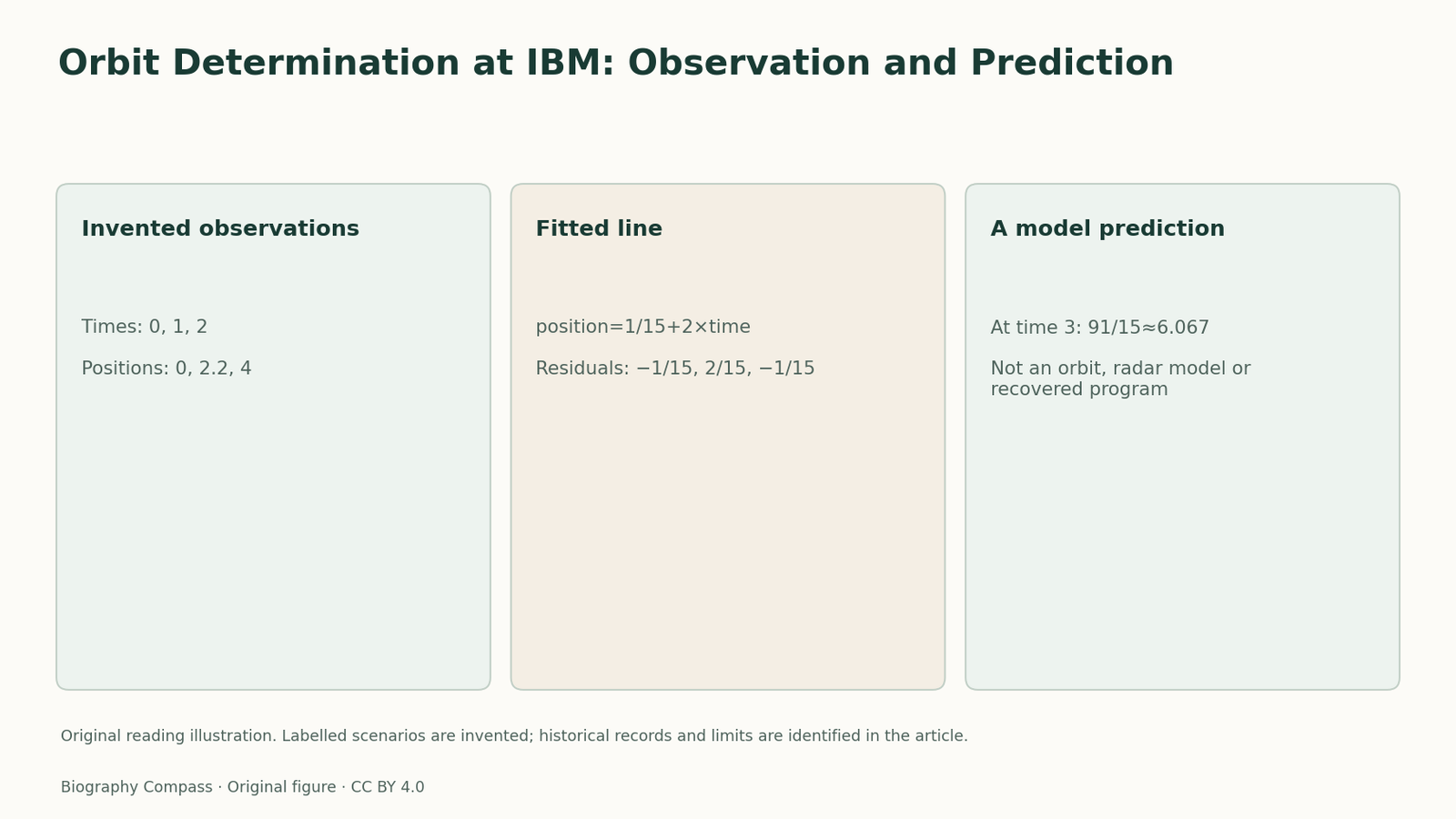
| Observation | The invented input at time 1 is 2.2. | It is supplied data, not produced by the fit. |
| Estimated model | The fitted line is position=1/15+2×time. | Its residuals need not be zero. |
| Prediction | At time 3 the line gives 91/15. | This is extrapolation under a stipulated model, not a new observation. |
Chronology
A timeline of the turning points
Selected historical record
The cited record supplies the historical starting point; the labelled examples below are original.
The selected IBM record
A. R. Mowlem’s 1960 seminar paper describes the IBM Space Computing Center’s programming system, data flow and computation and prediction of satellite orbits and lunar trajectories from observations. The consulted evidence is its catalogue record and original abstract/introductory extract, not a reading of the complete proceedings.
Granville’s biography places her in contractor teams doing space-related computation. Mowlem is the named author of this paper. Linking the two provides an industry context; it does not identify her as the author of this report or of every program described by it.
An original fitting example that is not an orbit
Invent three one-dimensional measurements: at times 0, 1 and 2, positions are 0, 2.2 and 4. Assume, solely for this teaching example, the model position=a+b×time and choose a and b to minimize the sum of squared residuals. The mean time is 1 and mean position is 31/15. The fitted slope is 2 and the intercept is 1/15.
The fitted positions are 1/15, 31/15 and 61/15. Taking observed minus fitted gives residuals −1/15, 2/15 and −1/15. The model does not pass exactly through every observation. That is consistent with the stated fitting goal. These inputs and this straight-line model are invented and do not represent orbital dynamics, radar geometry or an IBM historical algorithm.
Prediction adds distance from the evidence
At time 3, the fitted line predicts 91/15, approximately 6.067. No observation at time 3 was supplied. The value is therefore a consequence of extending the model, not a fourth measurement. A different assumed motion law could agree with the three observations and disagree later.
This small example shows the logical distinctions without claiming a realistic space-flight calculation. Actual orbit determination requires suitable physical and observational models; a line fitted to one-dimensional positions is not a substitute. The historical abstract establishes the kind of work the centre discussed, not the precise method used in this invented exercise.
What to ask of a tracking claim
Identify the observations, the reference time, the chosen motion model and the method used to estimate it. Then separate fit residuals from errors in future predictions. A small residual on the input data does not guarantee a small forecast error. A graph labelled “trajectory” may contain measurements, fitted values or predictions, and the label should say which.
Those questions give readers a concrete way to examine space-computing history without attributing an uninspected program to a famous individual. The reference answer is a transparent arithmetic illustration, while the record’s author, scope and attribution limits remain explicit.
Continue the chronology
Related history guides
Biography context
Explore United States through connected lives
Connected biographies
A working life behind the record
1924–2023
Evelyn Boyd Granville
Mathematician and educatorScientific computing and educationRead biographyQuick answers
Common questions
- Is the straight-line calculation a reconstruction of Granville’s space software?
- No. It is an original non-orbital fitting example. The available record does not identify it with her code or with Mowlem’s implementation.
Primary and institutional sources
How this history was checked
The account identifies the selected portions actually consulted. Original scenarios and reference answers explain the distinction without reproducing the source’s diagrams or implying that historical software was run. This article was reviewed on 5 November 2026.