
The short answer
A visible cusp makes a large theorem approachable, but it also creates a trap: a successful local calculation may be mistaken for the theorem itself. Compare two chosen equations and keep three questions separate: transformation, smoothness and the arrangement of the exceptional set.
Compare the evidence
Three checks that should not be collapsed
The distinction is between the question asked and the evidence needed to answer it.
| Question | Evidence or calculation | What remains open |
|---|---|---|
| Substitution | Compute total and strict transforms | Does not by itself prove smoothness |
| Gradient | A: (−1, 0); B: (0, 0) at the origin | A pointwise check in one chart |
| Exceptional intersection | For A, u = v² is tangent to u = 0 | Smoothness alone is not normal crossings |
Chronology
A timeline of the turning points
Characteristic-zero breakthrough
The global result exceeds the classroom fixture.
Compare two curves
Inspect the transform and the exceptional intersection separately.
The global question behind the local picture
Hironaka’s result concerns algebraic varieties over characteristic-zero fields in arbitrary dimension. The IMU memorial describes a proper modification that leaves the smooth part unchanged.
Kollár’s selected lecture distinguishes resolution from stronger normal-crossing requirements and explains why local constructions must fit together globally. His later exposition is not the original 1964 proof.
The exercise below works over the complex numbers. It tests selected equations in one chart, not the existence or compatibility of all the modifications required by a general theorem.
Define the chart and the objects being compared
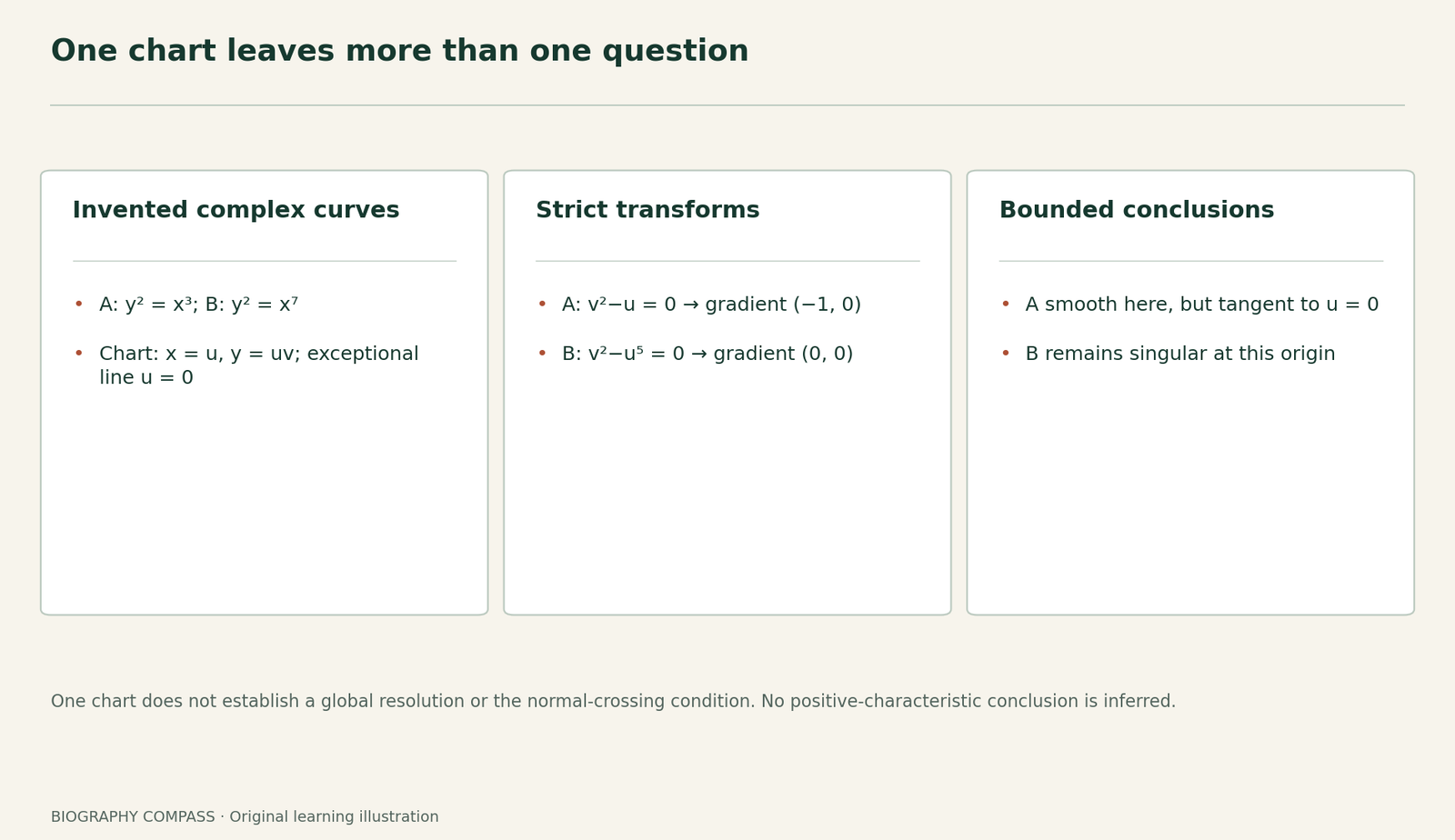
In one blow-up chart at the plane origin, write x = u and y = uv. The exceptional divisor in this chart is u = 0. Substitution gives a total transform; removing the common exceptional factor gives the strict transform.
For this exercise, use the plane-curve gradient test: a point on F(u, v) = 0 is smooth when the two first partial derivatives do not both vanish. Check only the origin of this chart. Other charts and intersections still matter to a global or embedded resolution.
Sources for this section: [2]
An original pair of curve calculations
Take curve A: y² = x³. After substitution, u²v² = u³, so the total transform is u²(v²−u) = 0 and the strict transform is v²−u = 0. Find its gradient at (u, v) = (0, 0).
Take curve B: y² = x⁷. The same substitution gives u²(v²−u⁵) = 0 and strict transform v²−u⁵ = 0. Calculate the gradient at the origin. Which strict transform is smooth there? Does smoothness alone establish a transverse intersection with the exceptional divisor?
Sources for this section: [2]
Reference answer: one improvement and two limits
For A the gradient is (−1, 2v), hence (−1, 0) at the origin: the strict transform is smooth there. For B it is (−5u⁴, 2v), hence (0, 0): a singularity remains in this chart.
A still meets the exceptional line u = 0 tangentially: writing u = v² gives tangent line u = 0 at the origin. Thus smoothness of that strict transform is not by itself a normal-crossing conclusion. B demonstrates that the same substitution need not finish even the local smoothing task.
Neither calculation checks the other chart, a complete sequence, global patching or the arbitrary-dimensional theorem. They are useful because they expose those separate obligations, not because they replace Hironaka’s proof.
Sources for this section: [2]
Continue the chronology
Related history guides
Tanaka: Soft Ionisation and Flight Time
Compare another research question with a bounded original worked example.
Read the timeline2008 account and an invented comparisonKitagawa: Frameworks and Gas Uptake
Compare another research question with a bounded original worked example.
Read the timelineBiography context
Explore Worldwide through connected lives
Connected biographies
Researchers connected with these questions
1931–2026
Heisuke Hironaka
Algebraic geometerHeisuke Hironaka studied singularities of algebraic varieties.Read biographyQuick answers
Common questions
- Does resolving one drawn cusp prove the theorem?
- No. A particular curve calculation cannot establish the global arbitrary-dimensional result.
Primary and institutional sources
How this history was checked
Selected original passages and the stated reading scopes support the historical account. Every teaching fixture is explicitly invented. This article was reviewed on 30 October 2026.